
Most inference software, including vLLM, SGLang, TensorRT-LLM and Triton, organizes work as discrete requests. A prompt arrives, the model runs, and the response ends. That model works well for request-driven LLM serving because the system can queue, batch and reschedule independent work.
Continuous inference has a different contract. The model keeps state and must advance on an external clock, such as the next audio frame, video frame, sensor update or control interval. Under concurrency, the request-serving stack misses this clock before the GPU’s compute capacity and memory bandwidth are fully used. We built the Wave Persistent Kernel (WPK) to fix that failure. In the workload measured here, .wave serves 56× more real-time sessions on the same GPU, with no missed deadlines.
Our first measured integration is NVIDIA’s Nemotron VoiceChat 11B. One beat contains two 80 millisecond model steps and has a 160 millisecond deadline. The chart below uses density for the number of sessions one GPU keeps on that schedule, and speed for the deadline divided by p99 latency. For a shorter account of the results, read the case study.
Figure 01 · Density × speed
Same GPU. 56× more real-time sessions.
Higher is better. Farther right means more conversations. At 1×, a beat finishes exactly at its deadline.
- WPK
- Reference stack (NIM)
- vLLM-Omni

WPK: 48 and 56 sessions measured; lower counts estimated. Session count is linear; speed is logarithmic.
Measurements, limits and physical-floor calculation
WPK: 140.0 ms p99 at 48 sessions and 147.5 ms at 56, the upper ends of the three-run ranges. The WPK points below 48 sessions are extrapolated, not measured. The two measured WPK points form the observed frontier; their connecting segment is a visual guide. Reference-stack points summarize three-run measurements at its Triton boundary; WPK includes its data plane. The floor is modeled device time, with no percentile. Each point uses its own deadline: 160 ms for WPK and NIM, 80 ms for vLLM-Omni. A speed of 1× means its p99 just fits that deadline; values below 1× miss it. The capacity ceiling is set at 56 sessions for this WPK profile, after allowing for a small memory reserve.
The floor cannot be reached by this real workload. It gives every operation peak chip throughput and perfect overlap without paying for instructions, synchronization or imbalance. Small matrix shapes cannot fill every arithmetic lane; memory transactions and pipeline dependencies leave bubbles. WPK removes much of the orchestration overhead, but it still pays these costs. A blue SM is executing work, not necessarily running at peak FLOP/s.
For every operation, divide its arithmetic by the H100’s dense peak at the required precision, and its modeled HBM traffic by peak bandwidth. Its ideal duration is the larger of those two times. A dependent operation starts only when its inputs are ready; independent branches may overlap.
F is arithmetic work, P is peak compute at the required precision, B is bytes moved, and β is peak bandwidth. e is the earliest ideal finish time; pred(i) contains the operations that must finish before i can start.
The beat must also fit the total work through the one chip. Its lower bound is the maximum of the total compute time, total bandwidth time, and longest dependency path. Shared weights are counted for the cohort; session state scales with the number of sessions.
- Compute
- 14.6 ms
- HBM bandwidth
- 53.5 ms
- Dependency path
- 52.5 ms
- Physical floor
- 53.5 ms
How request inference compares. Large, well-shaped prefill matrix multiplies can approach their compute roofline more closely because they provide enough parallel work and amortise setup. Small-batch autoregressive decode is usually more bandwidth constrained. Neither gives one universal “percent of peak” for a whole request. NVIDIA’s matrix-multiplication guide and GPU performance guide explain the shape, latency and instruction costs missing from an ideal roofline.
Our one-session reference-stack capture makes that distinction concrete: 30.5 ms of summed kernel time is about 2.1× the 14.7 ms modeled one-session floor, while its 119 ms server execution range is about 8.1×. The recorded WPK beat at 56 sessions is 143.0 ms against a 53.5 ms floor, about 2.7×. These describe different cohorts and timing boundaries, not a matched speedup. WPK’s gain is fitting many more sessions into the deadline, while still leaving a substantial gap to ideal hardware execution.
At 56 sessions, two causal steps per beat and 1,500 steps of history. The operation and traffic inventory uses the emitted Nemotron graph. Rates: 989 TFLOP/s BF16, 494.5 TFLOP/s TF32, 66.9 TFLOP/s FP32 and 3.35 TB/s HBM, using NVIDIA’s H100 SXM specifications at dense rates. This is an optimistic lower bound under that traffic and precision model, not an attainable schedule: it excludes host work, launch overhead, on-device coordination and imbalance, and assumes ideal overlap. Calculation data and assumptions.
One clock, many live sessions
Nemotron VoiceChat is one concrete example of continuous inference. It listens and speaks at the same time, often called full-duplex voice. Every 80 milliseconds it receives a frame of the user’s audio and produces a frame of its own. It runs whether or not anyone is talking, and its state, the memory of the conversation, grows for as long as the session lasts. A server does not hold one such session; it holds as many as it can, all live at once.
The same execution problem appears wherever a model maintains state and must advance on an external cadence. Streaming speech recognition, live translation, continuously generated video and always-on agents differ in what they compute, but not in this constraint: the next beat arrives whether or not the previous one is ready.
Request inference is usually measured in tokens per second and time to first token. Neither describes a session that must produce its next update on a recurring deadline. The measure that matters here is how many sessions one GPU keeps on schedule. We call it density. A session costs one GPU-hour divided by density, so density is the price of the product.
For the measurements in this article, real time means every 160 millisecond beat is served within 160 milliseconds of its schedule. Density is the largest number of sessions for which that holds, with zero late beats, across three consecutive runs.
A predictable beat needs a tight tail. p50 describes the typical beat; p99 shows the slower beats that can interrupt a conversation. In WPK’s full-context development run, p50 was 148.09 ms and p99 was 149.15 ms: just 1.06 ms, or 0.72%, apart. Keeping the schedule on the GPU removes repeated host submissions and scheduling decisions between operations, reducing sources of jitter.

Why the standard stack falls short
The standard way to serve a model is a framework that runs it as a sequence of GPU kernels, launched one by one from the host, wrapped in a server that schedules requests. It is a good design for requests. On a continuous workload it fails in five specific ways, and each of them shows up in a measurement.
Launches and the work between them. Small GPU kernels can finish before the host submits the next operation. In the reference stack, one captured 160 ms request for one session executes 3,999 CUDA kernels. Their summed execution time is 30.5 ms; the server’s execution range lasts 119 ms. No CUDA kernel runs for 75 percent of that range, with the longest gap at 8 ms. Kernel count is not host launch-call count: a single CUDA graph launch can replay many kernels. Figure 02 shows the resulting pattern: repeated host handoffs in standard serving, and a dense resident GPU program in WPK.
Orchestration. VoiceChat is five models: a perception encoder, a hybrid Mamba-attention backbone, a text-to-speech transformer, a codec, and a recognition head for the user's speech. A framework runs them as stages, and between stages the host decides: it copies sampled tokens back, runs a turn-taking state machine, loops over recognition symbols, and hands the next stage to an engine in another process. When the next GPU operation depends on one of those host decisions, the device cannot start that operation until the host has made it and submitted the work.
Serialisation. Batching sessions together should amortise this. It only does if the stack actually batches them. With two sessions, the reference stack executes 6,604 kernels per request group, summed kernel time rises to 61.9 ms, and the GPU is still idle 73 percent of the time. The kernel count grows and summed kernel time roughly doubles, consistent with another largely separate session pass rather than a shared cohort pass.
The weight pass. The modeled weight traffic for VoiceChat’s two steps is about 47 GB per beat, or 14 ms at peak H100 HBM bandwidth. Serving sessions one at a time repeats that traffic for each session; serving them together shares it across the cohort. That repeated cost belongs to the serial server design. The physical floor in Figure 01 instead counts the whole cohort’s arithmetic and memory traffic at the chip’s peak rates, while preserving the model’s sequential dependencies. At 56 sessions the modeled floor is about 53.5 ms, well below WPK’s 147.5 ms p99. The gap includes instruction overhead, imperfect resource use and the host boundary. Some of it can be reduced; the ideal floor itself is not an attainable runtime for this workload.
Dynamic machinery for a static workload. Paged caches, schedulers, dynamic batchers and allocators exist because requests are variable: unknown length, unknown arrival, unknown lifetime. A fixed cohort of sessions on a fixed cadence has none of that variability. Every session needs the same memory, forever; every beat does the same work. The dynamic machinery adds latency variance and nondeterminism to a workload that needs neither.
Figure 02 · Anatomy of a beat
Keep the beat on the GPU.
Standard serving

WPK

This is why NIM’s speed in Figure 01 falls as sessions are added. Repeated per-session work consumes the available deadline: its p99 fits at one session, then drops below the 1× real-time boundary at two.
What a persistent kernel is
WPK’s answer has three parts. Keep orchestration on the GPU instead of returning to the host between operations. Advance compatible sessions as one cohort so a weight pass can serve all of them. And compile the schedule and memory layout before the workload begins, when the model’s recurring structure is already known.
A persistent kernel is launched once and never exits. WPK launches 132 thread blocks, one per streaming multiprocessor of the H100, and they stay resident for the life of the process. What they execute is not a kernel in the usual sense but a program: a fixed sequence of phases, where each phase performs one operation for every session in the cohort at once. The host's only job is to publish the input for the next beat and wait for the output of the current one. Between those two moments it touches nothing.
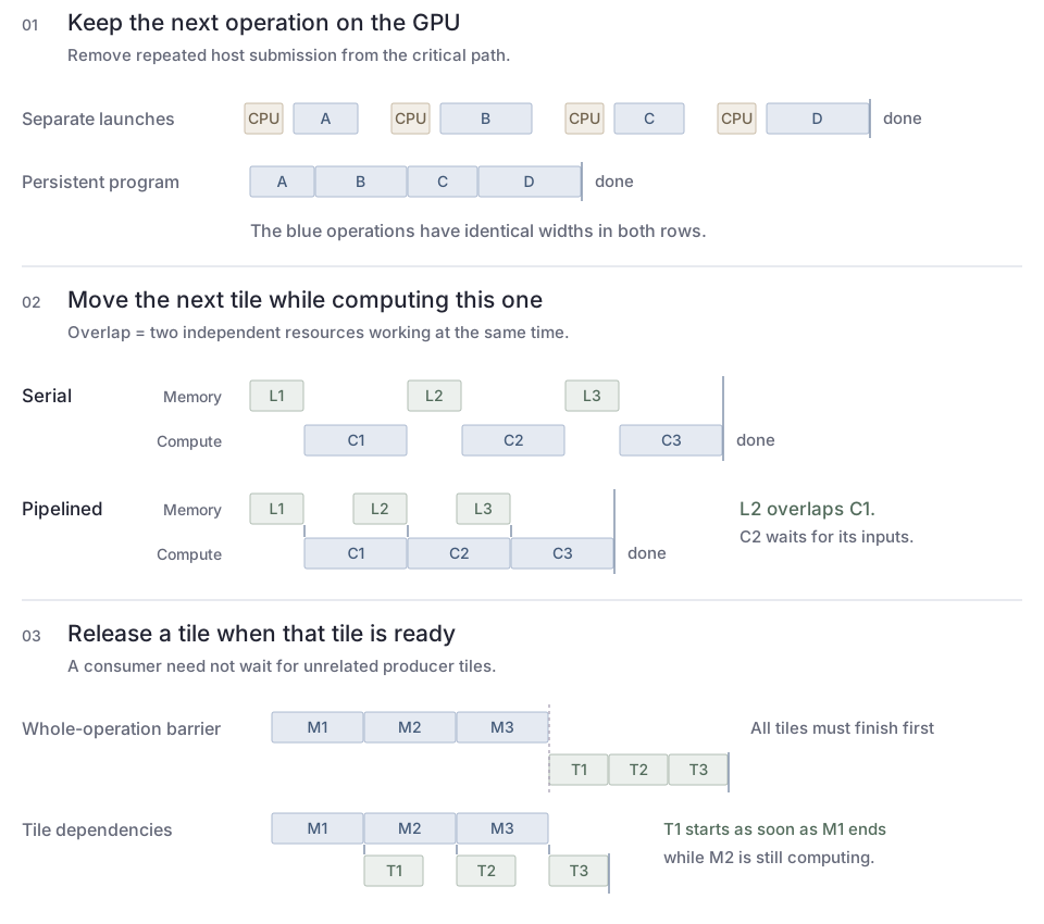
Why can the same operations run faster? Wall time includes the spaces between operations as well as the operations themselves. A resident program removes repeated host submissions. It can also keep a data-movement pipeline running across an operator boundary, and let a consumer use a finished tile while unrelated tiles are still being produced. Figure 03 separates those three effects.
Figure 03 · Why persistence helps
Same arithmetic. Less waiting between it.
Three general megakernel techniques. The widths of the work blocks stay the same; the schedule changes.
- Compute
- Load or transfer
- Host submission
L loads a tile; C computes it. M produces an output tile; T transfers that tile. Vertical guides mark when each tile is ready. The next weights may be fetched early, but an operation still waits for its input activations. The third example assumes compute and communication have resources to run concurrently. These original schematics explain the cross-task pipelining and fine-grained overlap discussed in the Mirage Persistent Kernel paper and No Bubbles.
Overlap means simultaneous progress on independent resources. Loading the next weights can happen while tensor cores use the current ones. A transfer can start when its own output tile is ready, without waiting for every tile in the operator. The arithmetic is unchanged; less of the memory and scheduling time lies on the critical path. Fusion can also keep intermediate values on-chip and avoid an HBM round trip. These gains require a suitable dependency graph, buffering and resource budget; persistence alone does not create them.
CUDA streams, graphs and specialized fused kernels can already exploit some of these opportunities. A megakernel makes the cross-operation schedule explicit inside one GPU program. WPK’s current design emphasizes a static cohort, shared weight passes and removing host orchestration.
One beat of VoiceChat at 56 sessions is 2,732 phases. In the three qualifying runs, p99 was 147.4 to 147.5 ms for the complete beat, including all five models and the data plane. Each phase applies its operation across the cohort, with weights shared between sessions and coordination kept on the GPU.
The weight pass illustrates what “together” buys. Under the traffic model, the approximately 47 GB read for each batch-one session becomes one shared pass for the cohort. Figure 04 isolates this reuse: weights are loaded tile by tile and applied to several sessions before moving on. This is a batching benefit that a conventional server can also capture if it truly batches the same model operations; persistence makes it part of WPK’s fixed beat program.
Figure 04 · Sharing the weight pass
Read a weight tile once. Use it for the cohort.
The same four sessions, drawn two ways. Sharing the pass reduces repeated weight reads; it does not make the sessions’ arithmetic or state disappear.
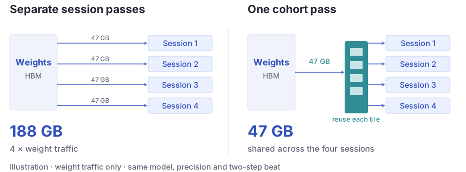
Figure 04 explains why density can improve without proportionally increasing weight traffic. It also identifies what to optimize in another server: batch compatible sessions at each weight-bearing operation. Reducing repeated weight traffic leaves more bandwidth for the growing cohort. Arithmetic, activations and per-session state still grow with it; WPK’s total beat remains above the physical floor in Figure 01.
At 56 sessions, WPK completes the full five-model pipeline and data plane within the 160 ms beat. Most of the work has a fixed cost per beat; only the text-to-speech attention grows with conversation length.
What disappears with the host out of the loop: launches, synchronisation points, the scheduler, the allocator. What has to exist instead: a static schedule that is correct by construction, because no runtime will catch a phase that starts before its inputs exist; fixed memory arenas for activations, state and weights, laid out at compile time; and a way to admit a new session at a beat boundary, which is a reset of one slot's state between two beats.
Persistent kernels are not new: persistent threads have long been used in graphics, including GPU ray tracing. They are attracting renewed interest for AI inference, with Hazy Research’s “No Bubbles” megakernel and Mirage Persistent Kernel (MPK) showing how a whole model can run as one GPU program.
WPK differs from those on four points, and the differences follow from the workload. The unit of work is a fixed cohort of independent sessions on a fixed cadence, not one sequence. The program spans five heterogeneous models in one kernel, with state that persists across beats for minutes: attention caches, recurrent states, rings and pages inside fixed arenas. The schedule is static and compiled, deliberately: there is no on-GPU scheduler, so the cost per session is flat and predictable, and the per-session isolation can be proven rather than assumed. And the objective is density at a deadline rather than latency of one sequence.
Why it needs a compiler
Writing and optimizing a persistent megakernel by hand for each model would mean repeatedly working out how to distribute operations across the GPU, respect their dependencies and reuse memory. Each change in session capacity or context length would require revisiting those choices. We built a compiler to automate that work: from a model expressed in Python Tensor IR and a library of CUDA operators, it generates the execution schedule and memory layout that drive the persistent kernel. Improvements to scheduling, memory reuse and shared operators carry across models and combine with one another. When a new model uses supported operators, integration can be quick: express it in the IR and validate its outputs, with little or no additional kernel engineering.
The model is expressed in Python using WPK’s Tensor IR. The compiler generates the tensor graph from that description, then lowers it into tasks and phases with explicit dependencies. CUDA operator bodies are implemented separately and reused across compatible shapes. The compiler checks the generated graph, binds each phase to an operator body and a physical shape, places the phases on the thread blocks with a cost model of bytes and flops, lays out every activation, every piece of session state and every weight in fixed arenas with storage recycled across lifetimes, and writes a 128-byte payload per phase with every pointer and stride. The result is a profile, one artifact per capacity, that the kernel loads once and executes beat after beat.
Figure 05 · The compiler
From model graph to running kernel
Python Tensor IR and CUDA operators. A generated graph, a compiled profile, and a GPU program that repeats every beat.

The compiler resolves operations, dependencies, worker assignments and storage before launch. At runtime, only input and output epochs cross the host boundary; the loaded program and session state stay on the GPU.
Experiment notes and measured results
Runtime and timing boundary
Between the kernel and the network sits a small runtime written in Rust. It keeps a fixed 160 ms clock. Packets arrive on each session's own schedule and are sequence-locked to beats; a packet is held one tick to absorb jitter, and if a packet has still not arrived when its beat must start, the runtime substitutes silence and starts on time, so that no session's network can stall the cohort. Sessions join and leave at beat boundaries, which is a reset of their slot between two beats. The kernel and the runtime exchange one 64-byte control record per beat, an input epoch and an output epoch, and every beat is timestamped at the boundary.
That runtime is what keeps the host out of the kernel's way, and it is where transport policy lives. It is deliberately simple. The public transport today is plain WebSocket, unoptimised; a real-time transport is planned. For that reason, the timing in this article is measured at the server boundary, and the transport's own behaviour is reported separately.
Protocol and measured results
Model, precision, inputs and timing boundaries used for the comparison:
- Same model. NVIDIA-NemotronLabs-VoiceChat-11B, one Hugging Face revision. Its 1,629 tensors match the reference stack's six-file server repository with zero mismatches; both load the same numbers.
- Same precision. bf16 perception and backbone, fp32 recurrent state, fp32 text-to-speech, codec and recognition, TF32 matrix multiplies, fp32 attention cache for the text-to-speech. These are NVIDIA's choices; WPK made the same ones.
- Same inputs, same scenario, same context. Every session: 40 seconds of silence, then an 80-second scored window containing the same recorded question, then 8 seconds of tail. About two minutes of context at the end of the window, inside the model's training envelope of 142 seconds and inside the two-minute context we configured for this VoiceChat build, so both systems attend over the identical history.
- The reference stack as shipped. The pinned NIM container, its shipping Triton configuration, its default two-step mode. Nothing tuned, nothing patched.
- Clocks at the server. Timing is taken on each pod at the server's own boundary. For the reference stack that is the Triton boundary with its WebSocket audio server bypassed, which excludes NVIDIA's own service layer and favours it. For WPK it is the data plane's per-beat record, which includes ours.
- Three consecutive runs per point, at least 100 tail samples per session, every failed attempt retained and counted, including our own two voided attempts on a lossy network path.
| System | Sessions at real time |
|---|---|
| WPK | at least 56, the highest tested |
| Reference stack, two-step, as shipped | 1, with one late request in 1,500 |
| Reference stack, one-step mode, latency reference | 1 |
| vLLM-Omni v0.28.0, native duplex path | no point established |
| System | Sessions | p99 | Late beats |
|---|---|---|---|
| WPK | 48 | 139.9 to 140.0 ms | 0 of 72,000 |
| WPK | 56 | 147.4 to 147.5 ms | 0 of 84,000 |
| Reference stack, two-step | 1 | 142 to 143 ms | 1 of 1,500 |
| Reference stack, two-step | 2 | 172 to 176 ms | 8 to 15 percent |
| Reference stack, two-step | 4 | 186 to 188 ms | 26 to 39 percent |
| Reference stack, two-step | 8, its configured maximum | 317 to 351 ms | most |
| Reference stack, one-step | 1 | 95 to 97 ms per 80 ms step | 0 |
| vLLM-Omni | 1 | 215 ms per 80 ms step | 18.5 percent, one run |
Three things to read from the tables. WPK's p99 moves 7 ms from 48 to 56 sessions, and across three runs it varies by a tenth of a millisecond; no beat in 156,000 exceeded its p99 by more than 0.7 ms. The reference stack's configured maximum of eight sessions is an admission limit, not a demonstrated density: at eight it runs at twice real time. And vLLM-Omni's native duplex path, in its shipping default, served each 80 ms step in 100 ms at the median at a single session, which is slower than real time; only one of its runs completed, the endpoint produces no user transcript in that configuration, and two attempts failed before scored work for reasons that may lie in our harness. We claim nothing for it beyond the observation.
What is next
WPK’s compiler is model- and modality-agnostic. We plan to validate the approach across other real-time workloads, starting with streaming automatic speech recognition (ASR).
Making these gains useful in an application also requires a service that teams can deploy without building and maintaining their own GPU serving stack. That is the purpose of WIM (Wave Inference Microservice), which we’ll introduce in a future release: a deployable service that packages the compiled model and its runtime.